Graph Structures#
PyTensor works by modeling mathematical operations and their outputs using
symbolic placeholders, or variables, which inherit from the class
Variable. When writing expressions in PyTensor one uses operations like
+, -, **, sum(), tanh(). These are represented
internally as Ops. An Op represents a computation that is
performed on a set of symbolic inputs and produces a set of symbolic outputs.
These symbolic input and output Variables carry information about
their types, like their data type (e.g. float, int), the number of dimensions,
etc.
PyTensor graphs are composed of interconnected Apply, Variable and
Op nodes. An Apply node represents the application of an
Op to specific Variables. It is important to draw the
difference between the definition of a computation represented by an Op
and its application to specific inputs, which is represented by the
Apply node.
The following illustrates these elements:
Code
import pytensor.tensor as pt

x = pt.dmatrix('x')
y = pt.dmatrix('y')
z = x + y
Diagram
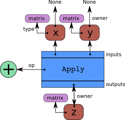
The blue box is an Apply node. Red boxes are Variables. Green
circles are Ops. Purple boxes are Types.
When we create Variables and then Apply
Ops to them to make more Variables, we build a
bi-partite, directed, acyclic graph. Variables point to the Apply nodes
representing the function application producing them via their
Variable.owner field. These Apply nodes point in turn to their input and
output Variables via their Apply.inputs and Apply.outputs fields.
The Variable.owner field of both x and y point to None because
they are not the result of another computation. If one of them was the
result of another computation, its Variable.owner field would point to another
blue box like z does, and so on.
Traversing the graph#
The graph can be traversed starting from outputs (the result of some computation) down to its inputs using the owner field. Take for example the following code:
>>> import pytensor
>>> x = pytensor.tensor.dmatrix('x')
>>> y = x * 2.
If you enter type(y.owner) you get <class 'pytensor.graph.basic.Apply'>,
which is the Apply node that connects the Op and the inputs to get this
output. You can now print the name of the Op that is applied to get
y:
>>> y.owner.op.name
'Elemwise{mul,no_inplace}'
Hence, an element-wise multiplication is used to compute y. This
multiplication is done between the inputs:
>>> len(y.owner.inputs)
2
>>> y.owner.inputs[0]
x
>>> y.owner.inputs[1]
InplaceDimShuffle{x,x}.0
Note that the second input is not 2 as we would have expected. This is
because 2 was first broadcasted to a matrix of
same shape as x. This is done by using the OpDimShuffle:
>>> type(y.owner.inputs[1])
<class 'pytensor.tensor.var.TensorVariable'>
>>> type(y.owner.inputs[1].owner)
<class 'pytensor.graph.basic.Apply'>
>>> y.owner.inputs[1].owner.op
<pytensor.tensor.elemwise.DimShuffle object at 0x106fcaf10>
>>> y.owner.inputs[1].owner.inputs
[TensorConstant{2.0}]
All of the above can be succinctly summarized with the pytensor.dprint()
function:
>>> pytensor.dprint(y)
Elemwise{mul,no_inplace} [id A] ''
 |x [id B]
 |InplaceDimShuffle{x,x} [id C] ''
   |TensorConstant{2.0} [id D]
Starting from this graph structure it is easier to understand how automatic differentiation proceeds and how the symbolic relations can be rewritten for performance or stability.
Graph Structures#
The following section outlines each type of structure that may be used in an PyTensor-built computation graph.
Apply#
An Apply node is a type of internal node used to represent a
computation graph in PyTensor. Unlike
Variable, Apply nodes are usually not
manipulated directly by the end user. They may be accessed via
the Variable.owner field.
An Apply node is typically an instance of the Apply
class. It represents the application
of an Op on one or more inputs, where each input is a
Variable. By convention, each Op is responsible for
knowing how to build an Apply node from a list of
inputs. Therefore, an Apply node may be obtained from an Op
and a list of inputs by calling Op.make_node(*inputs).
Comparing with the Python language, an Apply node is
PyTensor’s version of a function call whereas an Op is
PyTensor’s version of a function definition.
An Apply instance has three important fields:
- op
An
Opthat determines the function/transformation being applied here.- inputs
A list of
Variables that represent the arguments of the function.- outputs
A list of
Variables that represent the return values of the function.
An Apply instance can be created by calling graph.basic.Apply(op, inputs, outputs).
Op#
An Op in PyTensor defines a certain computation on some types of
inputs, producing some types of outputs. It is equivalent to a
function definition in most programming languages. From a list of
input Variables and an Op, you can build an Apply
node representing the application of the Op to the inputs.
It is important to understand the distinction between an Op (the
definition of a function) and an Apply node (the application of a
function). If you were to interpret the Python language using PyTensor’s
structures, code going like def f(x): ... would produce an Op for
f whereas code like a = f(x) or g(f(4), 5) would produce an
Apply node involving the f Op.
Type#
A Type in PyTensor provides static information (or constraints) about
data objects in a graph. The information provided by Types allows
PyTensor to perform rewrites and produce more efficient compiled code.
Every symbolic Variable in an PyTensor graph has an associated
Type instance, and Types also serve as a means of
constructing Variable instances. In other words, Types and
Variables go hand-in-hand.
For example, pytensor.tensor.irow is an instance of a
Type and it can be used to construct variables as follows:
>>> from pytensor.tensor import irow
>>> irow()
<TensorType(int32, (1, ?))>
As the string print-out shows, irow specifies the following information about
the Variables it constructs:
They represent tensors that are backed by
numpy.ndarrays. This comes from the fact thatirowis an instance ofTensorType, which is the baseTypefor symbolicnumpy.ndarrays.They represent arrays of 32-bit integers (i.e. from the
int32).They represent arrays with shapes of \(1 \times N\), or, in code,
(1,
None)
, whereNonerepresents any shape value.
Note that PyTensor Types are not necessarily equivalent to Python types or
classes. PyTensor’s TensorType’s, like irow, use numpy.ndarray
as the underlying Python type for performing computations and storing data, but
numpy.ndarrays model a much wider class of arrays than most TensorTypes.
In other words, PyTensor Type’s try to be more specific.
For more information see Types.
Variable#
A Variable is the main data structure you work with when using
PyTensor. The symbolic inputs that you operate on are Variables and what
you get from applying various Ops to these inputs are also
Variables. For example, when one inputs
>>> import pytensor
>>> x = pytensor.tensor.ivector()
>>> y = -x
x and y are both Variables. The Type of both x and
y is pytensor.tensor.ivector.
Unlike x, y is a Variable produced by a computation (in this
case, it is the negation of x). y is the Variable corresponding to
the output of the computation, while x is the Variable
corresponding to its input. The computation itself is represented by
another type of node, an Apply node, and may be accessed
through y.owner.
More specifically, a Variable is a basic structure in PyTensor that
represents a datum at a certain point in computation. It is typically
an instance of the class Variable or
one of its subclasses.
A Variable r contains four important fields:
- type
a
Typedefining the kind of value thisVariablecan hold in computation.- owner
this is either
Noneor anApplynode of which theVariableis an output.- index
the integer such that
owner.outputs[index] is r(ignored ifVariable.ownerisNone)- name
a string to use in pretty-printing and debugging.
Variable has an important subclass: Constant.
Constant#
A Constant is a Variable with one extra, immutable field:
Constant.data.
When used in a computation graph as the input of an
OpApply, it is assumed that said input
will always take the value contained in the Constant’s data
field. Furthermore, it is assumed that the Op will not under
any circumstances modify the input. This means that a Constant is
eligible to participate in numerous rewrites: constant in-lining
in C code, constant folding, etc.
Automatic Differentiation#
Having the graph structure, computing automatic differentiation is
simple. The only thing pytensor.grad() has to do is to traverse the
graph from the outputs back towards the inputs through all Apply
nodes. For each such Apply node, its Op defines
how to compute the gradient of the node’s outputs with respect to its
inputs. Note that if an Op does not provide this information,
it is assumed that the gradient is not defined.
Using the chain rule, these gradients can be composed in order to obtain the expression of the gradient of the graph’s output with respect to the graph’s inputs.
A following section of this tutorial will examine the topic of differentiation in greater detail.
Rewrites#
When compiling an PyTensor graph using pytensor.function(), a graph is
necessarily provided. While this graph structure shows how to compute the
output from the input, it also offers the possibility to improve the way this
computation is carried out. The way rewrites work in PyTensor is by
identifying and replacing certain patterns in the graph with other specialized
patterns that produce the same results but are either faster or more
stable. Rewrites can also detect identical subgraphs and ensure that the
same values are not computed twice.
For example, one simple rewrite that PyTensor uses is to replace the pattern \(\frac{xy}{y}\) by \(x\).
See Graph Rewriting and Optimizations for more information.
Example
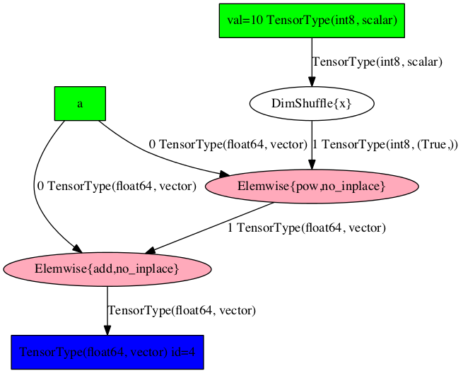
Consider the following example of rewrites:
>>> import pytensor
>>> a = pytensor.tensor.vector("a")      # declare symbolic variable
>>> b = a + a ** 10                    # build symbolic expression
>>> f = pytensor.function([a], b)        # compile function
>>> print(f([0, 1, 2]))                # prints `array([0,2,1026])`
[    0.     2.  1026.]
>>> pytensor.printing.pydotprint(b, outfile="./pics/symbolic_graph_no_rewrite.png", var_with_name_simple=True)
The output file is available at ./pics/symbolic_graph_no_rewrite.png
>>> pytensor.printing.pydotprint(f, outfile="./pics/symbolic_graph_rewite.png", var_with_name_simple=True)
The output file is available at ./pics/symbolic_graph_rewrite.png
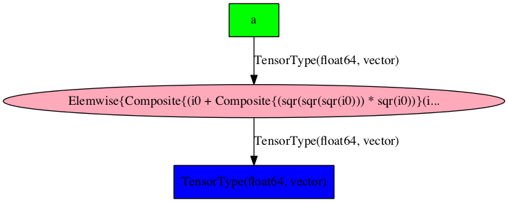
We used pytensor.printing.pydotprint() to visualize the rewritten graph
(right), which is much more compact than the un-rewritten graph (left).
Un-rewritten graph |
Rewritten graph |
|
|---|---|---|
|
|